3.2.  Simulink Interface for Octopus

Simulink is an interactive tool for modeling, simulating and analyzing dynamic systems. The MathWorks Inc., the leading developer and supplier of technical computing software, created it. Allowing interactive simulations, parameters can be changed “on the fly” and produce effects [Mat00].

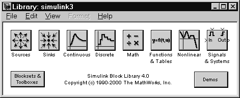
All Simulink Models have three things in common: They have some sort of signal generator, maybe more than one, that produce values subject to time. The values may represent physical variables, electrical systems or simply mathematical numbers. Second, the signals are processed through an arbitrary number of operations like integrals, gain blocks, and much others. The elements of such a Simulink model are called blocks. Figure 3.10 shows the block groups in Simulink.

With Simulink, one can simulate e. g. physical behavior like a bouncing ball, or automotive applications like an automatic transmission control, both presented with this thesis in a video demo, see appendix  4 on page 287 for details. The graphical user interface is one of the main benefits of Simulink. With drag-and-drop operations the user draws the models, like block diagrams. The blocks have the possibility to customize them, there are several variables for each block. It is also important that models are hierarchical, so it is possible to build models using both, top-down and bottom-up approaches. The user can view the system at a high level, then go down through the levels to see increasing levels of model detail. This approach, called sub block masking, provides insight into a model’s organization and how its parts interact [Mat00].

Basically, a Simulink block diagram is just a pictorial model of a dynamic system. It consists of a set of symbols, called blocks, interconnected by lines. Each block represents an elementary dynamic system that produces an output either continuously (a continuous block) or at specific points in time (a discrete block). The lines represent connections of block inputs to block outputs. The type of the block determines the relationship between a block’s outputs and its inputs, states, and time. A block diagram can contain any number of instances of any type of block needed to model a system. A block is the elementary dynamic system that Simulink knows how to stimulate. The output of a block is a function of time and the block’s inputs and states, if there are any. The particular function depends on the type of block.

There are stateful and stateless blocks. The integrator is an example for a stateful block, because the output depends on the history of the input. So its only state is the integral value before the current time. An example for stateless blocks is the gain block, which simply outputs its input signal, multiplied with a constant called the gain.

An important classification of blocks is, to divide them into continuous and discrete blocks. A continuous block responds immediately to continuously changing input. A discrete block, by contrast, responds to changes only at integral multiplies of a fixed sample time, holding its output constant in the meantime. Blocks that allow both working modes are called to have an implicit sample rate.

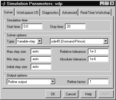
The actual simulation itself allows several customizations, too. For different purposes, different solvers can be used. The solver is the engine that involves the numerical integration of sets of ordinary differential equations (ODEs). There is a major difference between variable-step and fixed-step solvers and the meaning of these is already included in their names. For most solvers the minimum and maximum step size, and the tolerances can be tailored to the specific requirements of the simulation.

Scripting Simulink is possible, too, using the command line interface. Access is provided to all functions and settings, so scripts can automate simulations.