3.2.1.  Simulink S-Functions

Although there is a whole bunch of different blocks, there will always be the need for an engineer to use own, proprietary blocks that are not present in the library of Simulink. So there exists the capability to define blocks, using S-functions. These are computer language descriptions of Simulink blocks. An S-function can be written in MATLAB, C, C++, Ada, or Fortran. We will use C/C++ for our purpose. For usage in models, a block named S-function is dragged from the library into the model. Its dialog box takes the name of the S-function, which has to be also the name of the file, the S-function is compiled in. Additionally, there is a second field, taking the parameters that should be passed to the S-function.

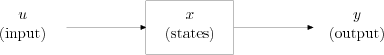
As all other blocks, S-functions process inputs u and states x to receive an output y. It is up to the S-function to perform this task by reacting to the callbacks Simulink invokes. These will be discussed below.

This diagram can be expressed using equations that show the mathematical relationship between the inputs, states and outputs, taken from [Mat01, p. 20].

3.2.1.1 Simulation stages

A Simulink model is executed in stages [Mat01]. The first one is the initialization phase, where Simulink incorporates library blocks into the model. Widths, data types and sample times are propagated, parameters are processed and the block execution order is determined. The second phase is the simulation loop. A single pass through the loop is called a simulation step. During a simulation step, Simulink executes all blocks by invoking functions that calculate states, derivatives and outputs of a block.

In Figure  3.13 on page 234 you see the execution stages that all blocks run through. Two terms were not mentioned before: Locate zero crossings is a mechanism that allows solving the problem that occurs when an input signal crosses the zero line. Many functions change their behavior and output dramatically when getting an input zero. In numerical simulation, as it is used here, normally the zero line is passed with the same step size as the rest of the simulation. But this could lead to a mis-behavior in the output vector. Simulink faces this problem by decreasing the step size when being near zero, to allow the model producing correct results. Minor time step is the part of the loop where outputs can be re-calculated. Here the zero crossing detection is done, too.

3.2.1.2 Callbacks and Concepts

The S-function has to provide a set of callbacks to allow Simulink directing the simulation. Subsequently there will be a list of the tasks, the callbacks perform:

Initialization.

This callback is invoked prior to the first simulation loop. It has to initialize a structure containing information about the S-function, called SimStruct. Then it sets the number and dimensions of input and output ports, and the block sample time or times. Finally, it allocates storage areas and arrays. The associated callbacks are mdlInitializeSizes and mdlInitializeSampleTimes for what the names suggest, then mdlStart for the startup process.

Calculation of next sample hit.

This function applies only when a variable sample time is used for the particular block. As the name suggests, it calculates the next step size, depending on state and current input. mdlGetTimeOfNextVarHit is the name of the function invoked for this.

Calculation of outputs.

The function mdlOutputs is called in every major time step to make all output ports valid.

Update discrete states.

Called in major time step, too, this ensures that all discrete states are in the state they have to be for next simulation loop pass. The associated callback is mdlUpdate.

Integration.

If a model has continuous states or non-sampled zero crossings or both, the minor time steps are evaluated, calculating output and derivatives. Two callbacks are used for the integration phase: mdlDerivatives and mdlZeroCrossings.

There are three key concepts that are important for implementing S-functions:

Direct feed-through.

If the output is controlled directly by the value of an input port, this is called direct feed-through. Two basic characteristics can indicate it: Either the output function mdlOutputs is a function of the input u, which means that u is accessed in mdlOutputs, or the “time of next hit” function mdlGetTimeOfNextVarHit accesses u.

Dynamically sized inputs.

Input dimensions to a block can be arbitrary; their size is determined dynamically in the initialization stage. The size then can lead to the number of continuous or discrete states, and the number of outputs. Dynamically sized inputs are very useful for attaching different sources to the block, e. g. a three-channel multiplexer that has a three-element output vector, or a clock that has a scalar output.

Setting sample times and offset.

This is the concept that explains how the block is acting in time. There are several different possibilities for timing:

Continuous sample time.

This kind of timing is used for S-functions that have continuous states and/or non-sampled zero crossings. The output changes in minor time steps.

Continuous but fixed in minor time step.

The S-function is executed at every major simulation step, but it does not change values in minor time step.

Discrete sample time.

The block acts as a function of discrete time intervals. Additionally, an offset can be specified for delaying the sample time hit. The effective sample time hit occurs at TimeHit = (n ⋅period) + offset, with n starting at zero.

Variable sample time.

This is a special case of discrete sample time, where the intervals between sample hits can vary. The variable sample times for the next hit are queried at the start of each simulation step – a fact that was complicating the implementation.

Inherited Sample time.

A block can have no inherent sample time characteristics and be dependent on its input or output. In this case, it has inherited sample time, which can be taken from either the driving block, the destination block, or the fastest block in the system.

The sample times are usually given in pairs of sample time and offset time. According to [Mat01], the valid sample time pairs are:

with the following definitions:

3.2.1.3 Build process

The build process of C MEX S-functions is basically not complicated. The source file, in which the callbacks are implemented, has to follow certain rules. So it has to include a given header, define mandatory callbacks and include C source files in the footer. The source file is then compiled and linked with the Matlab/Simulink libraries to get a dynamically loadable library (DLL). This DLL has to have exactly the same name as the included S-function has. Implementation

For the implementation of the Simulink-Octopus interface several tasks had to be accomplished and parts to be written:

• S-function interface
• Octopus simulator interface
• Time synchronization
• Data exchange

All tasks mentioned in this list will be discussed in the following sections on their own, although it is not always possible to explain one functionality without considering the other.